Quantum RAS Planning

Authors: Shashank Sanjay Bhat, Udaya Parampalli, Joseph West and Tansu Alpcan

NOTE: Equations represented are given twice in some cases to address visibility and accessibility.

Introduction

The Australian Army is forecasting an increased use and reliance on Robotics and Autonomous Systems (RAS) in the future battlespace.^[i] When this outcome is realised, the system will be characterised by many platforms operating autonomously or semi-independently. Two near term opportunities of RAS are logistics resupply and persistent Intelligence Surveillance and Response (ISR). Consider a scenario where hundreds of autonomous systems are performing both logistics resupply and ISR. Some platforms may be delivering ammunition, fuel and medical supplies to the forward forces, while others provide persistent surveillance over the areas of interest. As operational conditions change, supply priorities may shift, routes may become unavailable, and new threats may appear in previously low risk areas. Planners must continuously decide the allocation of the units to the tasks and how they should respond to changing circumstances. Existing planning methods within the Army rely on the Joint Military Appreciation Process (JMAP)^{[ii] [iii]}.  JMAP operates on the assumption that military capability bricks are grouped into manageable sizes e.g. a combat brigade is divided into battalions, which are in turn divided into companies and again divided into platoons. This hierarchical structure simplifies planning, requiring coordination only at the interfaces between subunits. However, in a future battlespace dominated by RAS, the assumptions upon which this structure is based breaks down.

Companies like Amazon Prime Air are exploring the use of aerial RAS platforms to distribute packages to customers with minimal human involvement^[iv]. These systems dynamically allocate tasks, reroute in real time and scale to thousands of current independent ‘missions.’ While this industrial use-case has clear parallels to logistic resupply in the field, the scale is well beyond the ability of current military planning processes. The scale of planning is likely beyond human capabilities. To fully realise the adaptability, persistence and distributed mass that RAS promises, automated planning tools are needed to support the decision making.  An optimal plan can be considered as an optimisation problem. In other words, such a plan would allocate resources, sequence tasks and coordinate movement within given constraints, to achieve a mission objective that could be described by an ‘objective function’. An objective function could be based on fuel consumption, operational risk, expected casualties or probability of mission success. As the number of assets, constraints or the complexity of the objective function increases, the optimisation problem becomes exponentially more difficult to resolve. Classical planning tools do not scale efficiently in such large scales, particularly under real-time, military pressures.

Quantum computing offers a potential breakthrough for solving large problems with exponentially large solution spaces. Unlike classical computers, quantum systems can explore large solution spaces simultaneously by using fundamental principles of quantum mechanics, namely superposition and entanglement. In Quantum computing, information is stored in quantum bits, or qubits. Superposition allows a qubit to exist in multiple states at the same time. Entanglement links qubits in such a way that the state of one cannot be fully described without reference to the other, even when they are separated.

Several algorithms such as Quantum Approximate Optimisation Algorithm (QAOA)^[v], Quantum Annealing.^[vi], Variational Quantum Eigensolvers (VQE).^[vii], and Quantum Walk^[viii]  have been developed with applications that enable combinatorial optimisation.In addition to these native algorithms, there have been developments in the quantum inspired classical algorithms. These include Quantum Inspired Evolutionary Algorithms (QIEA)^[ix], which mimic quantum algorithms to improve the performance of classical optimisation routines. These algorithms have shown promise in hardware constrained environments.

This article examines these quantum algorithmic approaches, assessing their theoretical foundations, practical strengths, and implementation constraints within the RAS context. While providing a comparative overview, it focuses on QAOA due to its broad applicability, and compatibility with near term quantum devices. This article includes translating a RAS planning problem into a Quadratic Unconstrained Binary Optimisation (QUBO) formulation followed by an Ising Hamiltonian and a detailed quantum circuit construction and analysis.

In addition, the article also assesses the contemporary quantum computing landscape, highlighting the existing capabilities in quantum hardware, coherence times, error rates and mitigation strategies. It also provides a trend path, employing the quantum computing equivalent of ‘Moore’s law’ to illustrate the growth strategies. This analysis provides a realistic timeline and feasibility assessment for practical efforts to plan and implement RAS within the Australian Army.

Background and Fundamentals

Classical Methods and Limitations

Classical methods for RAS planning can include heuristic algorithms like A* ^[x] and the Dijkstra's^[xi] algorithm. Also, such methods regularly make use of techniques such as genetic algorithms^[xii] and particle swarm optimisation^[xiii]. Linear and integer programming approaches with meta heuristic methods such as simulated annealing^[xiv] and tabu search^[xv] have also proven themselves to be useful applications. While useful for small scale problems, as the problem size grows these algorithms begin to face performance bottlenecks. Indeed, they are impractical to deal with the exponential rise in computational effort needed to explore vast solution spaces.  Further, as variables such as number of agents, tasks or waypoints increase, these classical methods become increasingly expensive to compute. And they are unable to deliver near optimal solutions within designated time frames. These scalability issues arise from the NP-Hard nature of the RAS planning problems. These limitations have motivated the search for alternative paradigms which can handle such scenarios more efficiently.

Quantum Computing Fundamentals

Quantum computing is one such alternative, rooted in the principles of quantum mechanics and different from the standard classical computing models^[xvi]. Unlike classical bits which process information using either 0 or 1, quantum computers use quantum bits or qubits. Qubits exhibit the property of superposition which enable them to represent multiple values simultaneously and to explore many solution spaces in parallel.

In addition to superposition, quantum computers also exhibit entanglement – a phenomenon where the state of one qubit becomes correlated with another, regardless of the distance. This allows the representation of complex; interdependent variables and this characteristic is particularly advantageous in tackling multi-agent RAS problems. Another foundational concept is quantum interference which enables the construction of desirable solutions while suppressing those that are suboptimal. This mechanism allows quantum algorithms to guide computations towards optimal answers in a more efficient manner than can be achieved through random exploration.

Despite all these advantages, quantum computing is not without its challenges. One of the primary issues is decoherence. This term refers to the loss of information that occurs when a quantum system, such as a qubit interacts with its surrounding environment. Quantum states are short-lived, which can lead to the collapse of superposition and loss of entanglement before errors set in. Because modern technology has not advanced beyond the noisy intermediate scale quantum (NISQ) era^[xvii], the hardware is prone to noise and operational errors. Therefore, quantum computing solutions must be accompanied by error correction and error mitigation strategies. Such limitations constrain the practical scalability of quantum algorithms but are the focus of ongoing research.

Quantum Algorithms for RAS planning

This section presents a deep dive of the key quantum algorithms relevant to RAS planning.

Quantum Approximate Optimisation Algorithm (QAOA)

QAOA is a hybrid quantum classical algorithm designed to tackle combinatorial optimisation problems by preparing quantum states that can approximate optimal solutions. It operates by alternating between two types of unitary operations applied to an initial superposition state: one is the cost circuit that encodes the objective function. The cost circuit encodes the ‘cost’ Hamiltonian.  Hamiltonian in quantum mechanics is defined as an operator which corresponds to the total energy of the system including both kinetic and potential energy. Another component is the mixer circuit that encodes the ‘mixing’ Hamiltonian. The mixer component enables exploration of the solution space, while the cost component guides the system toward better solutions by encoding the optimisation objective. In combination, these functions ensure that the solution space is as fully explored as possible^[xviii]. 

For a given depth parameter p, the QAOA state is constructed by the given equation below:

|ψ(γ,β)⟩ = ∏_k=1^p e^-iβ_kH_M e^-iγ_kH_C |+⟩^⊗n

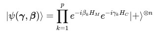
Here, γ=(γ₁, ... , γ_p) and β=(β₁, ..., β_p) are tunable parameters and ∣+⟩⊗n denotes an equal superposition of all the  basis states across n qubits. The algorithm aims to find the parameters (γ, β) which can minimize the expected value of the cost Hamiltonian with respect to the prepared state. The expectation value of the cost Hamiltonian is provided below:

E[γ,β] = ⟨ψ(γ,β)|H_C|ψ(γ,β)⟩

The expectation value is evaluated on a quantum processor, while a classical optimizer iteratively updates the parameters to converge towards an optimal solution. The algorithm is also compatible with the current NISQ devices, and its hybrid architecture allows for immediate applicability in practical workflows.

Quantum Annealing

Quantum annealing is based on the adiabatic theorem, which states that a quantum system will tend to be in its ground state if the corresponding Hamiltonian evolves slowly. Quantum annealing starts off with an initial Hamiltonian whose ground state is easy to prepare and slowly evolves to a problem Hamiltonian  which represents the objective function^[xix]. The time dependent Hamiltonian is expressed as:

H(t) = (1 − s(t))H₀ + s(t)H_C, s(t) ∈ [0, 1]

As t -> T, the system evolves to the ground state of , which is the optimal solution. Quantum annealers like D-Wave for example implement this process for QUBO based problems.

In the RAS domain, annealing is applicable to route optimisation, resource allocation and scheduling problems. The main strength of quantum annealing is that the associated hardware technology is relatively mature. Nevertheless, practical limitations remain, including noise sensitivity and the reliance on quantum annealers on predetermined optimisation scenarios.

Variational Quantum Eigensolver (VQE)

VQE is another hybrid quantum classical algorithm which was initially designed for quantum chemistry experiments. This algorithm estimates the ground state energy of a given Hamiltonian H by preparing a parametrised quantum state ∣⟩ and by minimising the expectation value given by the equation below:

E(θ) = ⟨ψ()|H|ψ(θ)⟩

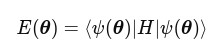
In the context of RAS, the Hamiltonian can be constructed from a QUBO model or any other cost representation to support scheduling, mission planning or resource usage. The optimization over is handled by a classical optimiser.

The algorithm is adaptable to near term quantum hardware and is able to handle complex cost structures. However, the utility of the algorithm heavily depends on the choice of the ansatz and the quality of the optimiser. Additionally, repeated circuit evaluations during parameter tuning can introduce computational overhead.

Quantum Walk Based Algorithms

Quantum walks are the quantum versions of classical mathematical process of random walks, characterised by superposition and interference. A discrete time coined quantum walk on a graph G(V,E) is described by the evolution operator equation below:

U = S · (C ⊗ I)

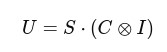
In this equation, C is a coin operator acting on the internal state of the walker, and S is the shift operator which updates the walker’s position^[xx]. By comparison to random walks, quantum walks enable faster diffusion through the state space and can be used for spatial search, path planning and information propagation.

In the context of RAS, quantum walks can explore large graphs such as navigation maps or coordination graphs among the agents. Their speedup offers a high dimensional planning^[xxi]. However, the algorithmic implementation remains complex and sensitive to decoherence.

Grover’s Search Based Algorithms

Grover’s algorithm provides a quadratic speedup for unstructured search problems by amplifying the amplitude of the marked states. For optimisation, Grover’s method is adapted by embedding the optimisation criteria to a quantum oracle O that flags optimal solutions. The Grover iteration is given by the equation below:

G = (2|ψ⟩⟨ψ| − I) · O

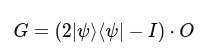
Here, ∣> is a uniform superposition of all the states. The number of iterations is approximately the order of O(N).

QAOA Problem Formulation for RAS Planning

RAS task planning problems could range from path optimisation for autonomous vehicles (or drones) all the way until multi-agent scheduling and coordination. In this context, it is useful to model a path optimisation problem as an optimisation task. For example, such a planning problem would be the structural equivalent of a traveling salesman problem (TSP) wherein a vehicle must visit a series of nodes exactly once and return to the origin point. In this scenario, the aim is to minimise the travel cost. There are benefits it conceptualising problems such as this as optimisation tasks via QAOA. QAOA leverages the QUBO formulation^[xxii] which is further mapped into an Ising Hamiltonian for encoding the problem into quantum hardware^[xxiii]. Below we detail the QUBO and the Ising Hamiltonian formulation by considering an example.

QUBO Formulation

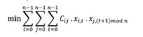
Given a cost matrix C where  represents the travel cost from node i to node j, the goal is to visit all the nodes which have the minimum total cost. Let  be a binary variable indicating whether node i is visited at time t in the tour. The total number of binary variables is , resulting in  qubits for the quantum computer. These variables are arranged in a matrix fashion where the rows represent nodes, and the columns represent time steps.

The objective function to be minimised is the total cost equation given below:

min ∑_i=0ⁿ⁻¹ ∑_j=0ⁿ⁻¹ ∑_t=0ⁿ⁻¹ c_ij · x_i,t · x_{j,(t+1)mod n}

To ensure a valid tour, some constraints are also added as penalty terms:

• Each node must appear only once:
  
• Each position in the sequence must be occupied by exactly one node.
  

Both constraints are added to the QUBO objective by adding large penalties A and B. The resultant penalty equation is shown below:

Q_penalty = A ∑_i=0ⁿ⁻¹ (1 − ∑_t=0ⁿ⁻¹ x_i,t)² + B ∑_t=0ⁿ⁻¹ (1 − ∑_i=0ⁿ⁻¹ x_i,t)²

The final QUBO matrix would be:

Conversion to Ising Hamiltonian

To run the QUBO matrix on quantum hardware, it is transformed into an Ising Hamiltonian. Here, binary variables are mapped into spin variables between the –1,1 value. Using the relation given below:

x = ^{1 − z}⁄₂

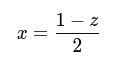
Substituting this back into the QUBO expression yields a Hamiltonian in the Ising form:

H = ∑_i h_iz_i + ∑_i<j J_ijz_iz_j

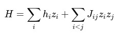
In this equation,  is a linear coefficient, and  is a quadratic coupling term between the spin variables. The resulting Ising Hamiltonian would represent the energy landscape of the problem. In this example, the minimum energy state would correspond to the optimal or near-optimal solution.

Qubit Projection for a Pure Quantum Solution

The number of qubits required to solve the problem scales non-linearly as the problem dimensions are encoded in the quantum space. Considering the most basic TSP, the formulation would use binary variables to represent whether a specific location is visited within a specific timeframe. This leads to quadratic scaling: n cities would require  qubits to represent all the city to position assignments. The same TSP can be extended to a vehicle routing problem (VRP) scenario^[xxiv] where there may be multiple vehicles operating simultaneously. To capture vehicle-to-city assignments we would require  qubits, where n is the city count, and v is the vehicle count. A vehicle-to-depot assignment would introduce an extra v.d qubits, where d is the number of depots. Furthermore, if there is a vehicle selection from a fleet of vehicles then we would need an extra v qubits for encoding the active vehicles. Similarly, if depot activation is also part of the problem, then we would need another d qubits. Summing all the components, the total qubit count would be: 

Total Qubits =

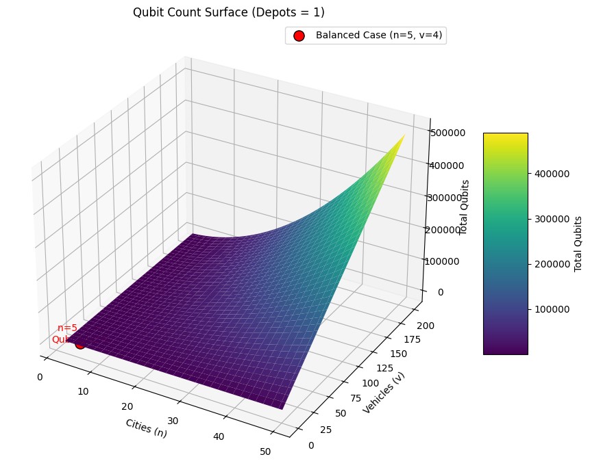
The surface plot in Figure 1 illustrates how the qubits grow with the problem size. For this simulation, the number of cities range from 1 to 100 and the number of vehicles range from 1 until 200. The number of depots is kept fixed at 1. The qubit count grows steeply for larger values of n and v. The scaling for cities is quadratic in nature. For the highest configuration (having 100 cities and 200 vehicles), the total projected qubit is approximately 500,000. Even under moderate scenarios such as 50 cities and 50 vehicles, the qubit demand exceeds 130,000 which is beyond the capability of current hardware. The red dot in the plot shows the scale of problems which can be tackled as a pure quantum formulation. For the current capability of 127 qubits a pure quantum solution could theoretically solve a balanced scenario of 5 cities, 4 vehicles and 1 depot.

Current Landscape and Future Projections

The commercial quantum sector has witnessed notable advances. Companies are pursuing a wide range of technological approaches which includes superconducting qubits, trapped ions, photonics and quantum annealing. All these developments demonstrate the ongoing efforts to improve qubit quality, increase system size and move towards a fault tolerant quantum computer. Notable examples from leading companies are outlined below: There are some impressive recent advances in quantum technology within the commercial sector. Some notable examples are listed below.

• IBM’s 433 qubit Osprey processor is already online.^[xxv] The company plans to introduce its first modular processor, Kookaburra, expected around 2026. This will be followed by the Cockatoo system in 2027, designed to interconnect multiple Kookaburra modules using L-couplers. These developments form part of IBM’s broader roadmap toward large-scale, fault-tolerant quantum computing, culminating in the Starling system, targeted for 2029^[xxvi]. At the time of writing, there were reports of the company integrating multiple dies into a 4158 qubit ‘Kookaburra’ module scheduled for late-2026 release^[xxvii].
• Google’s 105 qubit Willow chip has demonstrated the capacity to cross the break-even line for error correction, showing that a larger surface code patch can surpass the error rate of an individual superconducting transmon^[xxviii].
• Rigetti’s 84 qubit Ankaa-3 has the capacity to halve two qubit errors which is an improvement from its prior generation^[xxix]. This improvement also validates a multi-chip tiling strategy for the 336 qubit Lyra design.
• IonQ’s Forte registers 29 algorithmic qubits which is defined as the largest circuit size, outperforming any classical surrogate^[xxx]. Its 64 qubit Tempo, introduced around 2025, is now being progressively deployed to customers and research partners^[xxxi]. Quantinuum’s H-series has achieved the first logical qubit that outlives the best physical ion and posts a world record on a 20-qubit device^[xxxii].
• Photonic systems have reached quantum advantage in 2022 when Xanadu’s 216-mode Borealis gaussian Boson sampler produced a distribution in microseconds, an achievement which would have taken a classical hardware millennia to emulate^[xxxiii].
• While still in a pre-deployment phase, PsiQuantum have fabricated photonic chips on 300mm GlobalFoundries wafers, targeting one million physical photonic qubits and roughly one thousand logical ones around 2027^[xxxiv].
• DWave’s annealer employs more than 5000 flux qubits arranged in a Pegasus lattice. Testing has begun on a 7000 qubit and a 20-way connectivity Advantage 2 prototype in 2023. D-Wave has recently shown a measurable scaling speedup on a hard spin glass benchmark^[xxxv].
• Neutral atom ventures QuEra^[xxxvi] and Pasqal control 256-324 atom arrays today^[xxxvii].
• Microsoft’s “Majorana 1” nanostructure offers the first evidence of braiding ready zero modes which hint at topological qubits with gate errors below 10^-6^[xxxviii].

The Road Ahead

Moore’s Law in classical computing states that the number of transistors on a chip doubles every two years. While there is no formal qubit Moore’s Law, based on the relevant literature, we make an assumption that the qubit count doubles every 2 years and the average two qubit error falls by half for every hardware generation. We refer to this phenomena as “Qubit Moore’s law in this article.  At the 50-100 qubit level, error mitigated circuits tackle non-trivial chemistry and optimisation tasks. Once these numbers surpass approximately 1000 high fidelity physical qubits (or around 10 surface code logical qubits), opportunities will exist for early fault tolerant circuits such as deep phase estimation and error corrected QAOA on 256 variable instances^[xxxix].

Achieving this standard is already within reach of several technology companies. IBM plans to extend its exponential trajectory from 127 qubits beyond 10,000 qubits by 2027. Google has provided a six-milestone path to the first at-scale quantum computer by 2027. Willow is part of Milestone 2 which has already broken the logical error barrier^[xl]. IonQ expects 1024 algorithmic qubits by 2028 via photonic networking of modular traps^[xli]. Quantinuum projects approximately 100 logical qubits by 2027 and hundreds by 2029^[xlii]. Rigetti’s Lyra would deliver 336 physical transmons with less than a 0.5% two qubit error rate by 2026^[xliii]. PsiQuantum aims to reach one thousand logical qubits before the end of this decade. The success of its efforts will depend on factors such as the achievement of efficient fusion gates and ultra-low loss waveguides. The success of its efforts will depend on factors such as the achievement of efficient fusion gates and ultra-low loss waveguides^[xliv]. D-Wave remains on the annealing track by increasing qubit connectivity and integrating a gate-based spin qubit prototype^[xlv]. Neutral atoms aim to cross the 1k qubit threshold and demonstrate 128 logical Rydberg qubits by 2028^[xlvi].

Error Correction Trajectory

Superconducting qubit-based researchers are addressing known defects in the two-level system and moving towards a 3D chiplet packaging. The target is to reach coherence times above the 200-microsecond mark and the two-qubit error below 0.1% by 2027^[xlvii]. Trapped ion researchers have crossed the 99.9% qubit fidelity threshold on the next generation barium and ytterbium chain. This has been achieved by combining ultra narrow lasers and sympathetic cooling to support minute-scale coherence and sub 10^-3 logical error per surface code cycle. Photonic qubit researchers are driving silicon nitride to below the 0.1 dB m⁻¹ mark^[xlviii]. This is a key step for generating fusion based million qubit architectures. Neutral atom researchers are extending the optical-tweezer trap lifetimes by refining the stability of the Rydberg blockade towards a 99% fidelity^[xlix]. Topological qubit researchers are seeking to achieve at- hour scale coherence and two qubit errors below the 10^-6 mark. In summary, the milestone for all domains remains that physical qubits operate collectively as logical qubits.

Application Outlook

Quantum computers are expected to move beyond just a headline demonstration into multiple domains. Optimisation is the first domain which can be revolutionised using quantum algorithms. Hybrid gate based QAOA^[l] (or the next generation of D-Wave annealers) should be able to solve 100 to 256 variable routing problems^[li]. These problems would either be faster or achieve results closer to optimal than has been achievable using elite classical heuristics. In the cryptography domain, a million qubit fully error corrected machines remain a 2030’s goal. This aspiration should not ignore the fact that future generations of hardware could set even more impressive records. Factoring 100 plus bit RSA keys^[lii] or cracking smaller elliptical keys can be some of the achievements in the days to come^[liii]. Once this is achieved, scientific fields such as chemistry and material science will inevitably benefit from error mitigated VQE on a dozen high-fidelity qubits, enabling the achievement of chemical accuracy for medium molecules. In industries like agriculture and material science, such technology will accelerate battery and fertilizer design processes^[liv].

Beyond cryptography, in the domain of machine learning, 500 to 1000 qubits may embed quantum kernels into classical machine learning pipelines, fast linear algebra subroutines inside the classical pipelines which can yield speedups in classification problems^[lv].Once the hardware exceeds the 1000 qubit threshold (with suitable error correction) city scale traffic management will be within reach^[lvi].

Cost Perspective

Owning a quantum computer is an expensive affair. Estimates exist that it cost around 40 million euros over the period 2021-24 for Fraunhofer to install an IBM system One with ancillary infrastructure cost^[lvii]. The cost of D-Wave's 2000 qubit annealer is at 15 million US dollars. A standalone dilution fridge refrigerator can cost around 1-3 million US dollars^[lviii].

By contrast to owning a quantum computer, cloud access is far cheaper and has become an affordable option for many users. On Amazon Braket, a single shot on IonQ Forte costs 0.08 USD with a 0.3 USD task fee. The complete machine can be reserved for 7,000 USD per hour. Rigetti’s 84 qubit Ankaa costs 0.0009 USD per shot or 5,750 USD per reserved hour^[lix].

If we are to look at future perspectives, a 10,000-qubit machine would fall within the 1-2 billion USD range. This estimate considers the cost of infrastructure, hardware, installation, integration and the servicing costs^{[lx] [lxi]}. But this cost is likely to reduce over the years as quantum hardware matures, and quantum systems becomes more publicly available. Since the ADF may not need to use quantum algorithms frequently, it could access the technology with a cloud-based access setup and eventually shift towards owning a complete quantum computer once the technology has further matured and in response to its evolving needs. As the load and dependency towards a quantum solution increases, owning a computer becomes more cost efficient.

Conclusion

• The scale of planning required to effectively employ RAS platforms in the future battlespace will likely be intractable without new computational methods. The usage of quantum computing with RAS represents a paradigm shift in the way complex mission planning and multi agent systems are coordinated. Classical computational methods, while good for small-scale problems, become exponentially more complex as the task size and agent count increases. Quantum algorithms - which leverage the principles of superposition, entanglement and interference - offer a new approach. In short, quantum computers hold the potential to overcome classical computational bottlenecks.
• This article has explored multiple algorithmic approaches suitable for RAS planning such as QAOA, quantum annealing, VQE, quantum walk and Grover based methods. Every algorithm has a unique strength and suitability for specific types of RAS problems. For example, QAOA has hybrid adaptability and compatibility with NISQ devices. Annealing has hardware maturity and is fit for QUBO structured problems. Meanwhile, VQE allows for flexible parametrisation of cost functions. All these algorithms together enable a diverse toolbox for tackling a range of RAS applications.

The detailed explanation of QAOA (starting from the issue of problem encoding via QUBO to the Ising Hamiltonian and the circuit design) demonstrated its utility in solving complex optimisation tasks such as TSP and VRP. The qubit projection analysis further highlighted the scaling challenges for pure quantum solutions. As has been shown, even a moderate sized RAS problem can demand qubits which are beyond the capabilities of currently available hardware. The projections for advances in quantum technology showed the importance of hybrid quantum integration to achieving feasibility of using quantum technology in near-term.

The landscape of quantum computer hardware is evolving rapidly. Examples include IBM’s 400+ qubit processors, Google’s Willow processor and the emergence of photonic, ion trap, neutral atom and topological qubit technologies. The trajectory of qubit growth and error correction was also presented in detail. With the anticipated arrival of 10,000+ qubit systems by 2027, quantum hardware is on a path towards commercial and military deployment. Continuous research and innovation is required, however, to address challenges such as decoherence, gate fidelity and errors.

There are promising developments in the application of quantum technology. In the near term, quantum algorithms may offer speedups in solution quality for mid-sized routing and scheduling problems. In the longer-term, fault tolerant computers may emerge and problems such as city-wide autonomous traffic management, or large-scale RAS operations may become feasible. Cost dynamics suggest that cloud access is the most economically viable option for accessing quantum technology, especially for the military or other government sectors that are still exploring its potential uses. Over time, as hardware and use cases mature, government agencies may choose to acquire quantum computers for their own exclusive use.

In summary, quantum computing holds immense transformative potential for solving RAS planning problems. The practical realisation of this potential, however, requires a phased approach. For the ADF, this is likely to involve leveraging hybrid quantum classical algorithms before gradually transitioning towards a more comprehensive approach. This article lays the foundation for integration efforts and offers a roadmap for future exploration and adoption.

Endnotes

^[i] https://www.defence.gov.au/sites/default/files/2024-04/Factsheet-NDSOverview.pdf

^[ii] https://theforge.defence.gov.au/joint-military-appreciation-process-jmap-lite

^[iii]https://theforge.defence.gov.au/sites/default/files/adfp_5.0.1_joint_military_appreciation_process_ed2_al3_1.pdf

^[iv]https://www.aboutamazon.com/news/transportation/amazon-drone-prime-air-expanded-delivery-faa-approval

^[v] Farhi, Edward, Jeffrey Goldstone, and Sam Gutmann, “A Quantum Approximate Optimization Algorithm,” arXiv, November 14, 2014, https://doi.org/10.48550/arXiv.1411.4028.

^[vi] Tadashi Kadowaki and Hidetoshi Nishimori, “Quantum Annealing in the Transverse Ising Model,” Physical Review E 58, no. 5 (November 1, 1998): 5355–63, https://doi.org/10.1103/PhysRevE.58.5355.

^[vii] Alberto Peruzzo et al., “A Variational Eigenvalue Solver on a Photonic Quantum Processor,” Nature Communications 5, no. 1 (July 23, 2014): 4213, https://doi.org/10.1038/ncomms5213.

^[viii] Andrew M. Childs and Jeffrey Goldstone, “Spatial Search by Quantum Walk,” Physical Review A 70, no. 2 (August 23, 2004): 022314, https://doi.org/10.1103/PhysRevA.70.022314.

^[ix] Kuk-Hyun Han and Jong-Hwan Kim, “Quantum-Inspired Evolutionary Algorithm for a Class of Combinatorial Optimization,” IEEE Transactions on Evolutionary Computation 6, no. 6 (December 2002): 580–93, https://doi.org/10.1109/TEVC.2002.804320.

^[x] https://ai.stanford.edu/~nilsson/OnlinePubs-Nils/PublishedPapers/astar.pdf

^[xi] E. W. Dijkstra, “A Note on Two Problems in Connexion with Graphs,” Numerische Mathematik 1, no. 1 (December 1959): 269–71, https://doi.org/10.1007/BF01386390.

^[xii] https://www.jstor.org/stable/24939139

^[xiii]https://www.cs.tufts.edu/comp/150GA/homeworks/hw3/_reading6%201995%20particle%20swarming.pdf

^[xiv]https://www2.stat.duke.edu/~scs/Courses/Stat376/Papers/TemperAnneal/KirkpatrickAnnealScience1983.pdf

^[xv] https://link.springer.com/book/10.1007/978-1-4615-6089-0

^[xvi] Michael A. Nielsen and Isaac L. Chuang, Quantum Computation and Quantum Information: 10th Anniversary Edition, 1st ed. (Cambridge University Press, 2012), https://doi.org/10.1017/CBO9780511976667.

^[xvii] John Preskill, “Quantum Computing in the NISQ Era and Beyond,” Quantum 2 (August 6, 2018): 79, https://doi.org/10.22331/q-2018-08-06-79.

^[xviii] Leo Zhou et al., “Quantum Approximate Optimization Algorithm: Performance, Mechanism, and Implementation on Near-Term Devices,” Physical Review X 10, no. 2 (June 24, 2020): 021067, https://doi.org/10.1103/PhysRevX.10.021067.

^[xix] Edward Farhi et al., “Quantum Computation by Adiabatic Evolution” (arXiv, 2000), https://doi.org/10.48550/ARXIV.QUANT-PH/0001106.

^[xx] Dorit Aharonov et al., “Quantum Walks On Graphs,” 2000, https://doi.org/10.48550/ARXIV.QUANT-PH/0012090; Andris Ambainis, “Quantum Walk Algorithm for Element Distinctness,” 2003, https://doi.org/10.48550/ARXIV.QUANT-PH/0311001.

^[xxi] Childs and Goldstone, “Spatial Search by Quantum Walk.”

^[xxii] Kyungtaek Jun, “QUBO Formulations for Numerical Quantum Computing” (arXiv, 2021), https://doi.org/10.48550/ARXIV.2106.10819.

^[xxiii] Andrew Lucas, “Ising Formulations of Many NP Problems,” Frontiers in Physics 2 (2014), https://doi.org/10.3389/fphy.2014.00005.

^[xxiv] Victor Pillac et al., “A Review of Dynamic Vehicle Routing Problems,” European Journal of Operational Research 225, no. 1 (February 2013): 1–11, https://doi.org/10.1016/j.ejor.2012.08.015.

^[xxv]https://newsroom.ibm.com/2022-11-09-IBM-Unveils-400-Qubit-Plus-Quantum-Processor-and-Next-Generation-IBM-Quantum-System-Two

^[xxvi] https://www.ibm.com/quantum/blog/ibm-quantum-roadmap-2025, https://newsroom.ibm.com/2025-06-10-IBM-Sets-the-Course-to-Build-Worlds-First-Large-Scale,-Fault-Tolerant-Quantum-Computer-at-New-IBM-Quantum-Data-Center

^[xxvii] https://www.ibm.com/quantum/blog/ibm-quantum-roadmap-2025,

^[xxviii] https://research.google/blog/making-quantum-error-correction-work/

^[xxix]https://www.rigetti.com/news/rigetti-computing-launches-84-qubit-ankaa-3-system-achieves-99-5-median-two-qubit-gate-fidelity-milestone

^[xxx]https://investors.ionq.com/news/news-details/2023/IonQ-Forte-Launched-For-Commercial-Use-Making-AQ-29-Available-for-Customers-Worldwide/default.aspx

^[xxxi] https://ionq.com/quantum-systems/tempo

^[xxxii] https://www.quantinuum.com/press-releases/logical-qubits-start-outperforming-physical-qubits

^[xxxiii] https://xanadu.ai/blog/beating-classical-computers-with-Borealis

^[xxxiv]https://www.reuters.com/technology/startup-psiquantum-says-it-is-making-millions-quantum-computing-chips-2025-02-26/

^[xxxv]https://www.dwavequantum.com/company/newsroom/press-release/d-wave-demonstrates-first-ever-coherent-quantum-spin-glass-dynamics-on-more-than-5-000-qubits/

^[xxxvi] Jonathan Wurtz et al., “Aquila: QuEra’s 256-Qubit Neutral-Atom Quantum Computer” (arXiv, June 20, 2023), https://doi.org/10.48550/arXiv.2306.11727.

^[xxxvii]https://www.pasqal.com/newsroom/pasqal-unveils-a-new-quantum-processor-architecture-with-a-record-324-atoms/

^[xxxviii]https://azure.microsoft.com/en-us/blog/quantum/2025/02/19/microsoft-unveils-majorana-1-the-worlds-first-quantum-processor-powered-by-topological-qubits/

^[xxxix] Olivier Ezratty, “Is There a Moore’s Law for Quantum Computing?” (arXiv, March 27, 2023), https://doi.org/10.48550/arXiv.2303.15547.

^[xl] https://blog.google/technology/research/google-willow-quantum-chip/

^[xli] https://augmentedqubit.com/ionq-quantum-computing/

^[xlii]https://www.quantinuum.com/press-releases/quantinuum-unveils-accelerated-roadmap-to-achieve-universal-fault-tolerant-quantum-computing-by-2030

^[xliii]https://investors.rigetti.com/news-releases/news-release-details/rigetti-announces-new-partnerships-provides-business-updates

^[xliv]https://thequantuminsider.com/2024/10/21/pete-shadbolt-on-tackling-the-challenges-of-quantum-computing-its-future-impact-on-everyday-life/

^[xlv]https://www.dwavequantum.com/company/newsroom/press-release/d-wave-demonstrates-error-mitigation-on-the-advantage2-prototype-extending-coherent-annealing-range-by-an-order-of-magnitude

^[xlvi]https://www.quera.com/press-releases/quera-computing-releases-a-groundbreaking-roadmap-for-advanced-error-corrected-quantum-computers-pioneering-the-next-frontier-in-quantum-innovation-0

^[xlvii]https://www.ibm.com/quantum/assets/IBM_Quantum_Developmen_%26_Innovation_Roadmap_Explainer_2024-Update.pdf

^[xlviii] https://www.lionix-international.com/photonics/pic-technology/triplex-waveguide-technology/

^[xlix]https://quantumzeitgeist.com/harvard-mit-quera-achieve-historic-99-5-fidelity-in-quantum-computing-breakthrough/

^[l] Utkarsh Azad et al., “Solving Vehicle Routing Problem Using Quantum Approximate Optimization Algorithm,” 2020, https://doi.org/10.48550/ARXIV.2002.01351.

^[li] Humberto Munoz Bauza and Daniel A. Lidar, “Scaling Advantage in Approximate Optimization with Quantum Annealing” (arXiv, January 14, 2024), https://doi.org/10.48550/arXiv.2401.07184.

^[lii] Craig Gidney and Martin Ekerå, “How to Factor 2048 Bit RSA Integers in 8 Hours Using 20 Million Noisy Qubits,” 2019, https://doi.org/10.48550/ARXIV.1905.09749.

^[liii] Martin Roetteler et al., “Quantum Resource Estimates for Computing Elliptic Curve Discrete Logarithms” (arXiv, October 31, 2017), https://doi.org/10.48550/arXiv.1706.06752.

^[liv] Abhinav Kandala et al., “Hardware-Efficient Variational Quantum Eigensolver for Small Molecules and Quantum Magnets,” Nature 549, no. 7671 (September 2017): 242–46, https://doi.org/10.1038/nature23879.

^[lv] Aram W. Harrow, Avinatan Hassidim, and Seth Lloyd, “Quantum Algorithm for Solving Linear Systems of Equations,” Physical Review Letters 103, no. 15 (October 7, 2009): 150502, https://doi.org/10.1103/PhysRevLett.103.150502; Vojtech Havlicek et al., “Supervised Learning with Quantum Enhanced Feature Spaces,” Nature 567, no. 7747 (March 14, 2019): 209–12, https://doi.org/10.1038/s41586-019-0980-2.

^[lvi] Abyad Enan et al., “Optimal Traffic Flow in Quantum Annealing-Supported Virtual Traffic Lights” (arXiv, December 22, 2024), https://doi.org/10.48550/arXiv.2412.18776.

^[lvii]https://www.fraunhofer.de/en/press/research-news/2021/june-2021/fraunhofer-and-ibm-to-unveil-quantum-computer.html

^[lviii]https://www.theverge.com/circuitbreaker/2017/1/25/14390182/d-wave-q2000-quantum-computer-price-release-date

^[lix] https://aws.amazon.com/braket/pricing/

^[lx]https://patentpc.com/blog/the-cost-of-quantum-computing-how-expensive-is-it-to-run-a-quantum-system-stats-inside

^[lxi] https://quantumexplainer.com/how-much-does-a-quantum-computer-cost/