Subterranean Information from Gravity

Detecting Mass at a Distance

Author: Samuel Legge

This article is a deep dive into measuring gravity as a form of remote sensing and its potential applications in land warfare. It includes a tutorial on gravitational signals and an overview and projection of existing and future sensing technologies.

Introduction

Warfare has always involved a significant element of utilising underground infrastructure as a tactical asset. The resilience of the Ukraine forces entrenched in the extensive tunnel network of the Azovstal steelworks in Mariupol^[1] is a recent example of the strength of subterranean complexes; the Ukraine troops defended their position for months against a significant asymmetrical force. The most striking advantage afforded by subterranean structures, beyond the physical protection of layers of earth and rock safeguarding them against ordnance and direct assault, is their resistance to external observation. These structures are resilient to scans across the electromagnetic spectrum, which includes our most commonly used remote sensing methods such as radar, thermal imaging and multispectral analysis. This leads directly to our problem statement:

How do we remotely detect and gain information about subsurface operations and infrastructure?

This question becomes increasingly relevant as global urbanisation continues to shift the landscape of conflicts closer to cities and their associated subsurfaces. Below-ground tunnels in modern cities are complex networks of transport infrastructure (pedestrian, road and rail); piping and channels (supply, sewerage and stormwater); electrical and telecommunication utilities; mining tunnels; catacombs; and abandoned sub-infrastructure. The development of large tunnel-boring machines has continued to advance since the 1950s, with machines and tunnels both reaching diameters of over 10 metres; and globally an estimated 5,200 kilometres of tunnels are built every year.^[2] Even where well-documented subsurface maps of an area exist, their reliability will rapidly deteriorate if the area is subjected to conflict and bombing, with previously connected tunnels collapsing and alternative pathways being constructed.

One potential way of addressing the subsurface detection problem is by utilising gravity as a detectable signal. On Earth, we are very familiar with the strong gravitational attraction we experience; we are constantly pulled towards the planet’s centre at an acceleration of 9.8 m.s^‑2. Gravity is a fundamental physical force that is different from the electromagnetic force, and all mass produces a gravitational attraction that transmits through all known materials. Utilising this property, gravity can be used to ‘see’ changes in mass through the ground by detecting subtle variations in the gravitational field.

This technique, known as gravimetry, represents a unique sensing modality. It cannot be blocked, jammed or easily spoofed, making it particularly resilient in contested environments, and it is entirely passive, allowing silent detection in covert situations. Gravimetry is performed using a specialised sensor called a gravimeter, a highly sensitive type of accelerometer. While gravimetry remains a niche technology, it is widely used in geophysical resource exploration—typically in conjunction with other subsurface detection methods such as magnetometers, ground-penetrating radar and exploratory borehole drilling—to map geological structures.

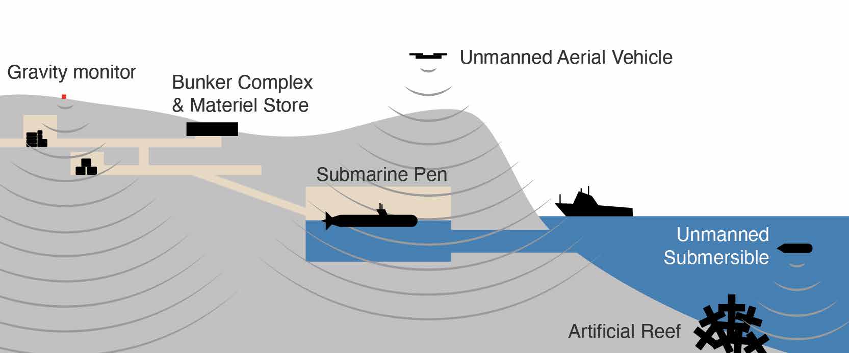
There are no documented examples of gravimetry being employed as a subsurface detection tool in active warfare. However, even existing commercial gravimetry technology holds potential relevance for military applications. For instance, a gravimeter could be deployed on the surface to detect the absence of mass caused by a tunnel or concealed bunker in a strategically important area, as illustrated in Figure 1.

Although these concepts can be tested using commercially available devices, their high cost and fragility may limit their suitability for use in active conflict scenarios. Nevertheless, ongoing advancements in gravimeter technology, particularly in the field of quantum sensing, are expected to produce next-generation devices that are smaller, more accurate, more robust and easier to operate.^[3] The following discussion investigates gravimetry in a device-agnostic manner and addresses its limitations, which are often hidden behind a ‘quantum complexity’ shield that allows new technology to avoid scrutiny of sensor performance and applicability to a particular use case.

From left to right, a surface-mounted gravimeter is used to map/observe near subsurface structures (detection and mapping achievable with current technology;, monitoring requires further technological development); a gravimeter-equipped airborne survey drone senses larger subterranean structures (requires further technological development); and an autonomous underwater vehicle silently measures local gravity to infer detailed ocean topography (requires further technological development). Conical green lines show the vision cone from each gravimeter.

This article will explore the application of gravimetry to the subsurface information problem through the following sections:

• Gravimetry Applications: a discussion of current and future applications of gravimetry relevant in both the defence and the civilian spaces
• Measuring Gravity: a tutorial on the mechanism of gravity, with an investigation of the generated signals from basic structures and the physical limitations of the method
• Gravimeter Technologies: an overview of gravity sensing technologies with a focus on the strengths, weaknesses and preferred applications of each, followed by a projection of future technologies
• Conclusion: the recommended future path for defence in this space. 

Gravimetry Applications

The idea of gravity detection is always the same: using the gravimetric signals generated by a nearby density variation to infer information about that structure or materiel below the surface. The technical capability required to achieve this is not insignificant, and will be discussed in greater detail in the following section. But for now, we will assume that we have a gravimeter above the area of interest and are looking to gather information, as depicted in Figure 1.

Subsurface Detection

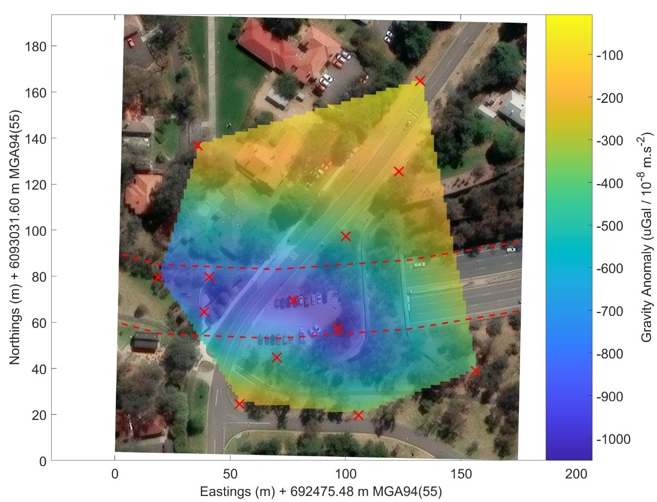
The simplest form of detection is a detection test—that is, using a gravity signal to confirm or deny the existence of a subsurface asset. An example might be when information is received that there may be an underground bunker in a particular area. In this case, if the area directly above this bunker is accessible, a gravimeter could do a two-point measurement to assess the likelihood of the structure’s existence. First, a nearby measurement would be made to establish the background gravitational field for that area, followed by a second measurement above the expected substructure. This kind of measurement can be visualised in Figure 2, which shows the measured gravitational signal generated by the Acton Tunnel from the surface.

This data was taken over two hours using a CG‑6 gravimeter^[4] and an Emlid RTK GPS.^[5] Red crosses indicate individual measurement points, and the interpolated colour map is generated from these points. Dashed red lines are indicative of tunnel/road position. Imagery data is provided by Maxar. The blurred gradient nature of the data is the expected result of this gravitational signal. The resolution of a gravitational ‘image’ is roughly equal to the depth of the signal, hence the highest possible resolution in this case is limited by the 20-metre depth of the tunnel.

Here, numerous surface data points were taken over the area to generate a rough map of the subsurface tunnel, with measurements directly above the tunnel, showing a decline in the expected value of local gravity of approximately 10^‑5 m.s^‑2 (this is a large signal for this kind of survey). For the CG‑6 gravimeter used to take this data in this scenario, a signal-to-noise ratio (SNR) of ~500 is achievable in a one-minute measurement.^[6] Verification of the tunnel’s presence via gravity could be done with only two measurements: first, a reference measurement on the road north of the tunnel to establish a baseline gravitational signal in that area; second, a measurement above the tunnel that would show the gravitational anomaly of the tunnel, confirming its presence. This application of gravimetry for land forces would be the simplest to implement; it’s fast and reliable, and can easily confirm or deny the existence of large subsurface infrastructure. However, difficulties arise if there is inconsistent subsurface geography, as changes in rock and soil types can mimic these signals. Additionally, if the chosen points are both directly above bunkers or voids, the signals may give a false reading. Because of these limitations, gravity is unlikely ever to be the single solution to a subsurface problem; instead, it is likely to be one sensing modality used in a broad-spectrum approach to detection.

Subsurface Mapping

Extending on the two-point measurement discussed above, greater knowledge of the subsurface structure can be gained by recording gravity at multiple sites above the site of interest. In this case, the gravimeter data is used to map out the area, as has been done in Figure 2.

In Figure 2, the continuation of the tunnel can be seen in the westerly direction (indicated by the blue shaded area), following its path as it traverses under the ridge. The resolution of this data is limited as the ground level is approximately 20 metres above the tunnel, effectively setting a 20-metre resolution of the subsurface structure. The strength of gravimetry for mapping is most effective when the gravimeter can be physically closer to the source. The actual detection limits of current gravimeters are dependent on the size, depth and density contrast of the subsurface structure but, as a rough estimate, in common rock/soil, at 1 metre below the surface, commercially available devices could detect a roughly 0.6 cubic metre void. Detection limits will be discussed in further detail in the ‘Measuring Gravity’ section.

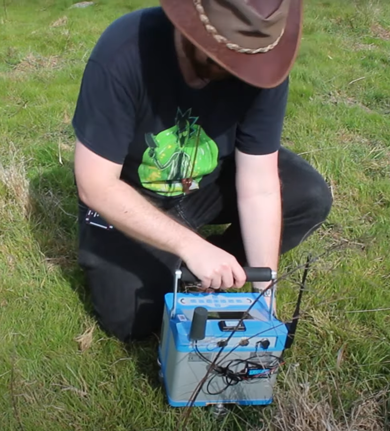
If we reconsider the drone deployment case shown in Figure 1, this distance limitation indicates the first clear physical constraint of this technology: the higher the drone is flown above the signal of interest, the lower the resolution of the signal that it can measure will become. It is not like a camera: there is no gravitational lens that can be used to image gravity at a distance. In addition, the signal strength decreases with distance, and the motion of the drone itself can severely degrade the gravity signal. These gravity sensing issues are intrinsic to the physical nature of gravity itself; they cannot be solved or sidestepped by any level of technological advancement or quantum sensing development. In almost all cases, the optimal solution would be for the drone to act like a grasshopper, flying and landing to make a gravity measurement grid of the area on the ground. Currently, such surveys are done using human-carried gravimeters similar to the Figure 3 example. Airborne gravimetry is possible, and actively performed using human-piloted, light fixed-wing aircraft in the geophysical surveying space, and drone deployment is an expected future development as gravimeters reduce in weight and size.

Subsurface Monitoring

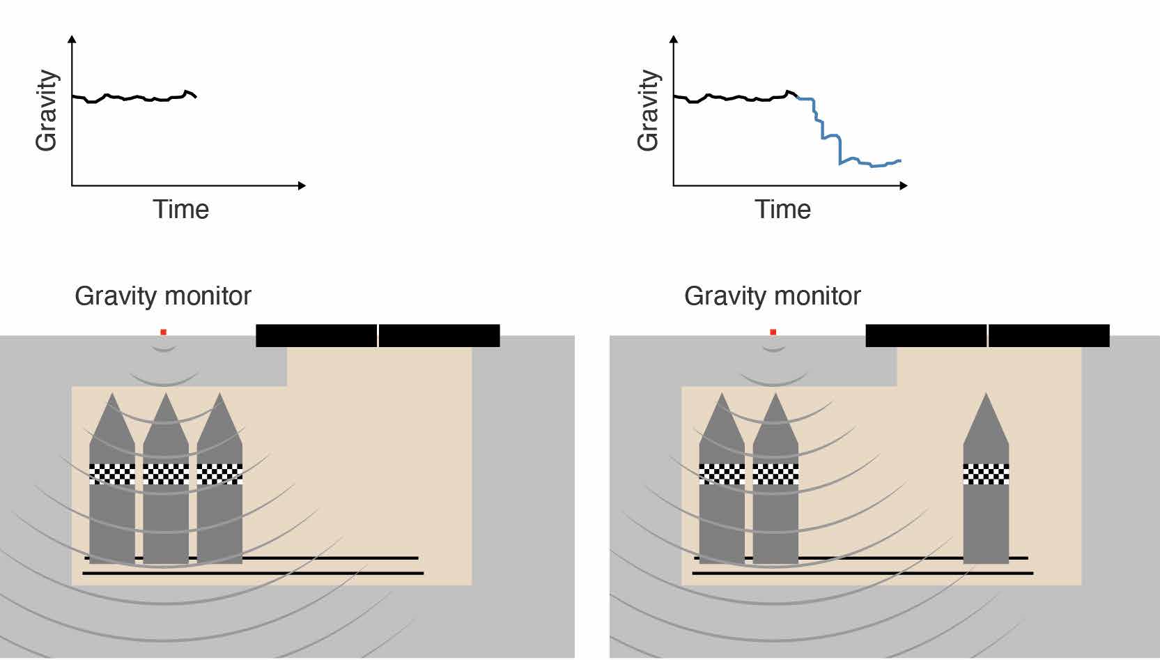
The final subsurface detection modality is active area monitoring. This can be thought of as using gravimetry to monitor a single point or an area for changes over time. In the examples discussed so far, the data has directly measured Earth’s gravity over the points of interest. These measurements show the data at a single time. However, if data were taken periodically over these areas as a differential measurement, any significant mass changes in the subsurface would become visible. This differential measurement method highlights changes between scans and would, for example, reveal any new tunnels that have been dug in the area since the previous dataset was taken. One could also imagine static gravity monitoring above a known cache where, if the materiel were sufficiently massive and close enough to the surface, its gravitational signal could be used to assess movements and cache levels as depicted in Figure 4. What is detectable via gravity is, again, dependent on the distance between the gravimeter and the target of interest, and the total mass of the target.

For current gravimeters, a good rule of thumb is the inverse square law (discussed in the ‘Measuring Gravity’ section) and the 100 kilograms at 1 metre distance rule—that is, if the object is 1 metre away, it should weigh at least 100 kilograms to be detectable. It follows then that if the object is 10 metres away it would need to weigh 10,000 kilograms to be detectable, and at 100 metres away it would need to weigh 1,000,000 kilograms to have a detectable gravity signal. These mass and distance constraints impose significant limitations when it comes to the kinds of materiel that could be monitored with gravity.

A significant limitation of the current gravimeters for this application is their lack of long-term stability. Commonly used commercial devices are based on a spring-type measurement that can drift at 2×10^‑7  m.s^‑-2/day,^[7] which would appear like a change in mass of 300,000 kilograms at a depth of 10 metres. In this case, the long-term stability of quantum sensors could be a significant improvement for this application. A gravimeter that has this long-term stability is typically known as an absolute gravimeter and can be thought of as a calibration-free device, measuring with atomically reference definitions of the second and the metre.

Navigation and Mapping

Of interest to combined land and naval forces, especially for littoral operations, is the ability of gravity signals to elucidate information about the ocean floor. Our current deep ocean floor maps are generated from gravitational data measured by airborne gravimetry and orbiting satellites (inferred through orbital changes, which have much worse resolution than terrestrial surveys).^[8] However, on a smaller scale, there is a strong focus following the 2023 Defence Strategic Review^[9] on the Indonesian archipelago and littoral operations. While not the only option for mapping the ocean floor, gravimetry is well suited to an uncrewed submersible that can passively detect the ocean topography with no active sonar or noise. It would be especially well suited to the detection of changes in ocean floor structure through differential measurement of an area over time. An example of this is depicted in Figure 1, where a submersible is used to identify the presence of an artificial reef, which might indicate pre-conflict effort to secure a beachhead area or secure a key asset from littoral invasion.

Another essential aspect of gravimetry to the defence forces is the necessity of a local gravitational map or model to remove local acceleration in the inertial navigation (IN) equation. The current reliance of all Australian forces on the global navigation satellite system is a known vulnerability, and the reliability of IN is an alternative to outside-in positioning. However, IN has a drift problem, whereby the longer you operate only on IN, the greater the circle of uncertainty as to where you actually are becomes. The advent of better gravimeters may also allow new techniques that solve this issue through gravitational map matching^[10]—that is, using pre-known gravitational anomaly signposts to correct to a known position.

This technique is comparable to the age-old method of positioning with a compass bearing and visible landmarks. By using known gravitational anomalies in the earth’s fields, they can act as landmark signals or ‘signposts’ to zero your position. This is particularly well suited to a submersible craft where there are minimal other signals to reference off. The impact of this technique has high value to naval and air platforms, but the direct applicability to land forces is lower, as there are typically easier to observe and measure sources of navigation signposts (such as local topography) when operating on land.

Table 1 summarises the defence applications of this technology, listing the technical requirements and difficulties of each and their likely impact on land forces. The technical difficulties are given for existing technologies; these will be more fully explained in the ‘Measuring Gravity’ section of this article. 

Table 1. Overview of defence applications for gravimetry

Application	Measurement time/constraints	Technical difficulty / principal factor/requirements	Impact/value
Subsurface detection	~5 minutes	Easy Portable gravimeter with short-term (two-point) stability. Single axis. Precision requirement set by target mass and depth. Achievable with current technology	Medium Validation of existing data
Subsurface mapping	~1 hour per 100 m2 (resolution dependent)	Hard Portable/drone-deployable gravimeter with short-term (survey-length) stability. Single axis. Precision requirement set by target mass and depth. Achievable with current technology	High Generation of new data
Subsurface monitoring	Long-term stability required	Very hard Gravimeter with long-term (absolute) stability. Precision requirement set by target mass and depth. 5–10-year technology horizon	High Generation of real-time data
Ocean floor mapping	~1 hour per 100 m^2 (resolution dependent)	Hard Gravimeter with long-term (absolute) stability. Full tensor gravity/gradient measurement desirable. 10-year technology horizon	Medium Generation of new data for littoral areas
Gravity map matching	Detailed pre-existing gravity maps required	Very hard Gravimeter with long-term (absolute) stability. Full tensor gravity/gradient measurement desirable. 10-year technology horizon	High Particularly for submersible platforms

 The following sections discuss civilian and commercial use cases of gravimetry, both established and emerging, and are included so that the reader knows the dual-use avenues of this technology and the areas where it is likely to be advanced outside military applications.

Mineral Exploration

Mineral and mining exploration surveys (geophysical surveying) are currently the largest established market for gravimeters. Gravity signals are generated by density variations in large subsurface ore deposits and are measured either by airborne gravimetry with fixed-wing aircraft close to the ground, or by ground surveys with human operators. The gravity data is typically used with other detection modalities, such as magnetic sensors and seismic reflectometry, to find potential deposits. This modality is very similar to the previously discussed subsurface detection and mapping applications; however, it typically looks at much deeper and volumetrically larger density variations than would be of interest to Army. The existing knowledge in this field of combining detection modalities and calculating the mass density inversion could be adapted for smaller-scale subsurface structures of interest in defence applications. Another application in this field involves using gravimetry to monitor deposits over time, a method that is often used for oil and gas reservoirs where the gravity over the field changes as the resources are pumped out and depleted. Again, this is an analogue to the subsurface monitoring application at larger scales and depths.

Construction/Archaeology

Analogous to subsurface detection and mapping, gravimetry has applications in civilian construction for areas with unknown subsurface structures. Underground voids, both naturally occurring or from historic structures, are a significant problem in the construction industry, often causing delays and, at worst, structural instability. As the cost and capabilities of gravimeters improve, gravimetry is likely to see more significant utilisation as a tool to detect and mitigate the risk in this field; gravity is particularly well suited to detecting possible sinkholes.^[11] Similarly, discovering buried voids in historical structures has archaeological applications where gravity is appealing as a detection modality, as it can passively identify substructures without disturbing the potentially fragile structures.

Groundwater/Volcanology

Measuring and tracking the use of groundwater as a resource is a difficult task, typically done by digging boreholes in the areas of interest. However, boreholes only provide a single data point for that particular location. The idea to utilise gravity as a catch-all mass sensor for near-surface groundwater is still being researched^[12]—its greatest challenge being the requirement of absolute gravimeters (gravimeters with long-term stability) to measure the groundwater signals over timeframes ranging from months to multiple years. At a deeper and larger scale, gravimeters have also been used in research to monitor active seismic areas such as volcanoes, where researchers use gravimeters to track changes in the subsurface magma environment over time.^[13]

Measuring Gravity

This section of the article will discuss the nature of gravimetric signals in detail, especially their limitations and constraints—which, given our current understanding of physics, restrict the potential applications regardless of sensor types or technological developments. By necessity, it is written at a higher technical level and gives a brief introduction to the underlying physics of gravimetry and precision measurement. The detail of this section will enable readers to make their own assessment about potential gravimetric signals in specific applications.

Fundamentals of Gravity

As previously discussed, a key property of gravity is that the signal (or field) travels unimpeded through all known material as well as the vacuum of space. This property makes it ideal for subsurface detection. However, it also means that there is no conceivable technology that allows us to manipulate gravity in a way that would let us refocus the signal at a distance, as we are accustomed to with optical technology. In the electromagnetic spectrum, where a lens or antenna can be used to manipulate light or radio, it is possible to image something at a distance, as is done in a typical camera. With gravity, there is no known technical pathway or physical possibility of creating a gravity lens, and therefore there is no way to focus the signal into a sharp image of what is underground. Instead, we measure a blurred signal from all nearby gravity sources. It is like having a camera that is always out of focus: you can’t see the image of what is in front of you, but it is still possible to detect the presence and relative brightness of different light sources. This is the primary reason why the gravitational signal of the tunnel in Figure 2 does not have sharp, well-defined edges. Even if more data points were taken, since the tunnel is 20 metres below the surface, the resolution will be limited to the distance of the signal from the sensor. This is a generally applicable rule of thumb for gravity mapping: the resolution limit will be the same as the distance between the source and the sensor.

The strength of a gravitational signal can be estimated by using the point mass approximation (where an object is approximated to its total weight located at its centre of mass). The acceleration due to gravity, g_z (or vertical gravitational signal), where the sensor is directly above the source, is given by

g_z = GM/r²

where G is the gravitational constant (6.67×10^‑11 N.m².kg^‑2), M is the object’s mass (kg), and r is the distance (m) of that object from the sensor. The SI unit for acceleration and, therefore, gravity is metres per second squared (m.s^‑2). Another popular unit in literature is the Gal (short for Galileo), where 1 Gal = 0.01 m.s^‑2, often used with SI prefixes with milli or micro (e.g. 1 µGal = 10^‑8 m.s^‑2).

The total gravitational signal can be calculated as the sum of individual mass sources, such that the gravitational force measured by a gravimeter is the total sum of all sources in their respective directions. Spherical sources of gravity can be perfectly modelled with the point mass approximation (this is known as Gauss’s law). These properties mean that we can calculate Earth’s gravity as a large, constant signal (spherical source at a distance) and estimate local changes in gravity as the sum of nearby signals of significance causing slight perturbations in the gravity field.

By this logic, the absence of mass can generate a local gravitational signal—that is, the presence of an underground room could be detected from the surface due to the reduction in local gravity caused by the removal of materiel, as shown in Figure 1. For example, if we assume a homogenous ground density of 2,700 kg^‑3, and a 20 m³ room 4 m below the surface, we can approximate this room as an effective negative mass of –54,000 kg, and if we use the above equation we get a signal of −2.3×10^‑7 m.s^‑2, indicating we expect a reduction of local gravity by this magnitude on the surface.

So far, we have only discussed the concept of gravity as attracting downwards, towards the centre of the earth. However, gravity is a three-dimensional vector field that has a component in all three orthogonal directions. For example, a vector gravimeter can measure acceleration in all three orthogonal directions (typically denoted g_x, g_y and g_z as the accelerations in the north, east and down directions) and could, for example, measure the attraction of a large mass such a mountain pulling you sideways very slightly. One of the biggest advantages of a vector gravimeter is the removal of the requirement to level the sensor so that the single measurement axis is aligned with the direction of the desired measurement. Currently, all commercially available gravimeters only measure in one axis (g_z, vertical), and require levelling at each measurement site.

Gravity Gradients

Gravity gradients are a commonly used extension to traditional gravity measurements, and operate on many of the same principles. The primary advantage of a gradient measurement is immunity to platform motion, but it also enables a slightly higher resolution detection of shallow density variations. However, the gradient signals are typically weaker and less useful in finding larger or deeper structures compared to a standard gravity survey.

By measuring gravity at multiple locations (either in sequence or simultaneously), it is possible to calculate the spatial rate of change of gravity, known as the gravitational gradient. There is a gradient of all three orthogonal vector components of gravity in all three orthogonal directions, totalling nine total values.^[14] The gravity gradient is typically denoted as G_** with subscripts indicating the gravity direction and the gradient direction; e.g., G_zz is the rate of change of g_z in the z or vertical direction, whereas G_zx is the rate of change of g_z in the x direction.

The simplest gravity gradient to consider is the vertical gravity gradient in the vertical direction, G_zz. The gradiometer sensor can be thought of as two gravimeters stacked vertically, one above the other, and the measurement is the difference in gravity between the sensors divided by the distance between them. The equation for the vertical gravity gradient signal with the sensor directly above the source is given by

G_zz = 2GM/r³

where G is the gravitational constant (6.67×10^‑11 N.m².kg^‑2), M is the object’s mass (kg), and r is the distance (m) of that object from the sensor. It should be noted here that the gravitational constant G (italicised) is different from the gradient G_zz. The units of a gravity gradient signal are accelerations per metre. This equates to units of m.s^‑2.m^‑1 = s^‑2 where the metre cancels such that the final unit is per second squared. The gravity gradient is commonly measured in Eötvös (E) where 1 E = 10^‑9 s^‑2.

If the gradiometer is fixed to a moving platform, any platform motion is common to both sensors and will be cancelled out of the final measurement. This is a key advantage of a gravity gradiometer and the primary reason why they are typically deployed on airborne surveys.

While gravity gradient measurements are inherently immune to platform motion, the signal of the gravitational gradient is typically much weaker than the direct gravity signal; the power falls with the inverse cube of the distance instead of the inverse square, resulting in lower measurement sensitivity. In addition, as the device is effectively two gravimeters, the complexity is increased and user operation is more difficult. Because of these factors, gradiometers are rarely used in land-based surveys.

Estimating Gravity Signals

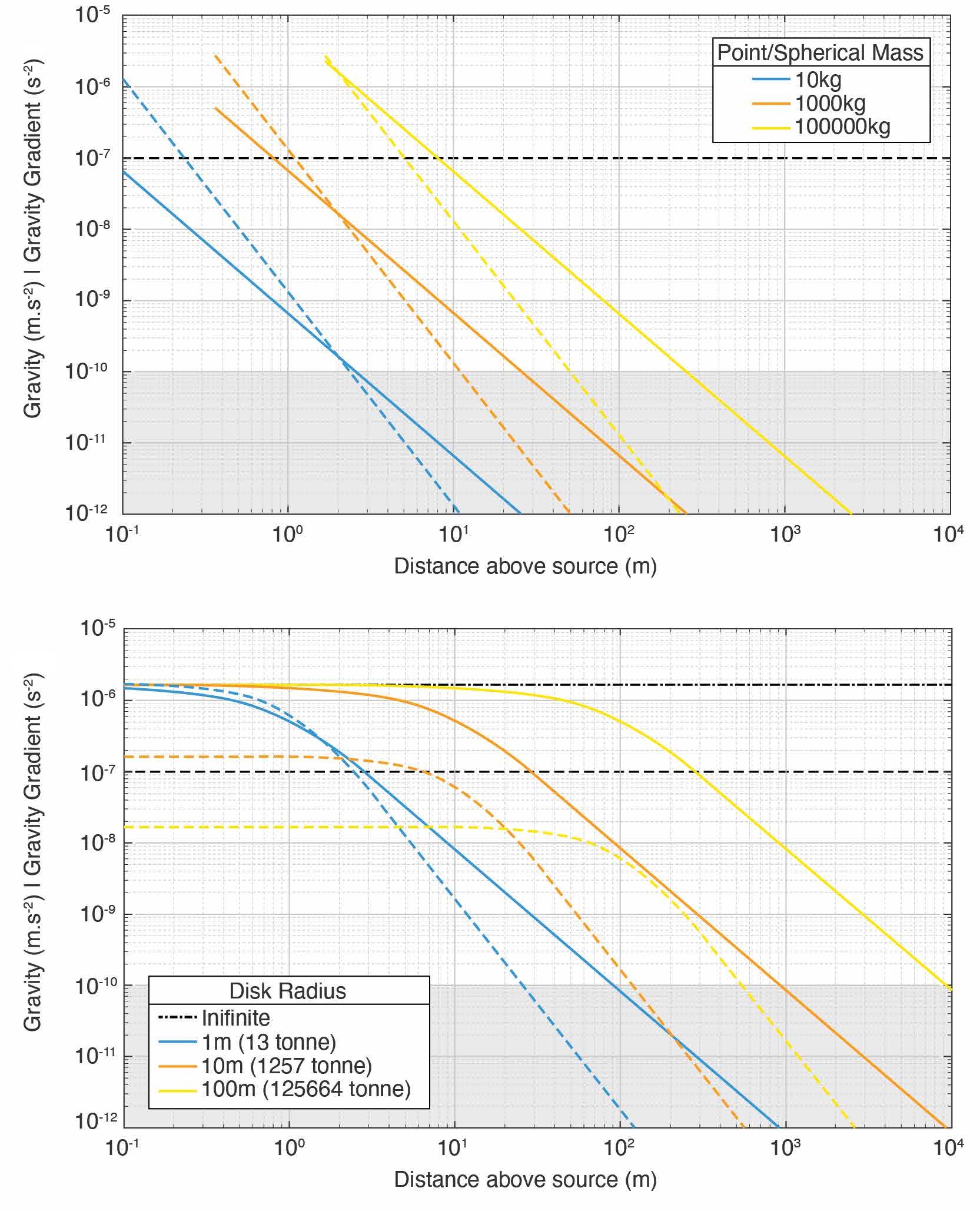
It is interesting to consider what kinds of gravitational signals can be generated from various structures. As mentioned, Gauss’s law means that any spherical source is equivalent to a point mass source, and for objects whose average radius is further away than their distance, this becomes an excellent approximation of the gravity signal that the object generates. For objects with a radius larger than their distance to the sensor, the gravitational signals become more complex but can often be approximated as a disk-like source, and the gravitational attraction is constant with distance until the spherical approximation can again be made. Figure 5 shows the gravitational and vertical gravity gradient signals for spherical sources of different mass and disks of various sizes. Here, the gravity response is flat close to the disk and then falls off with the inverse square law above the disk radius.

Another feature in Figure 5 is the flat gravitational signal generated by an infinite plane, as shown by the black dot-dashed line. Here, the gravity signal is limited by the density variation and thickness of the plane, and it is a more realistic representation of expected signals of any subsurface structures that are larger than they are deep.

The grey area at the bottom of the plots in Figure 5 is known as the sea of problems— systematic and random errors.^[15] Effectively, this is the expected lower floor of terrestrial gravity signal, where one of the limiting factors for earth-based measurements is the earth noise floor. The inherent noise of the ground (effectively the vibrations of the planet, known as the microseism) begins to limit the ability of sensors to measure below 10^‑10 m.s^‑2.

A gravity signal larger than 10^‑7 m.s^‑2 is detectable with commercially available gravimeters (CG‑6 with SNR of 10), shown as a horizontal dashed black line on the plots in Figure 5, and a gravity gradient signal larger than 10^‑8 s^‑2 is detectable with commercially available gravity gradiometers.

 

Assessing Gravimeter Specifications

Now that it is clear how to make an estimate of a gravitational signal, the question becomes, ‘Does a gravimeter capable of measuring that signal exist?’ The most important specifications for gravimeters, and the ones used to answer this question, are their precision and accuracy. The terms precision, stability, accuracy, sensitivity and uncertainty are often confused or misused when discussing measurements and are explicitly clarified here. When reading about or discussing weak signals such as gravity, it is important to check or clarify the intended message and ensure that the difference between accuracy and precision has not been lost.

Precision is synonymous with stability, sensitivity or variance, and can be thought of as the ability to make repeated measurements and get the same results reliably. An example is the grouping of shots when aiming at the same point, as demonstrated in Figure 6.

Accuracy is synonymous with uncertainty or drift, and can be thought of as the confidence that the values measured are correct. To use the same example, this is the average distance of shots from the point of aim or centre of target from an incorrect zero in the sights.

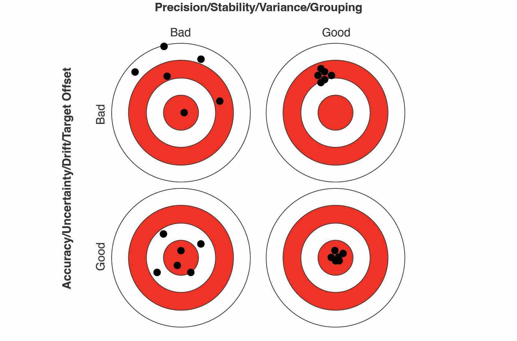
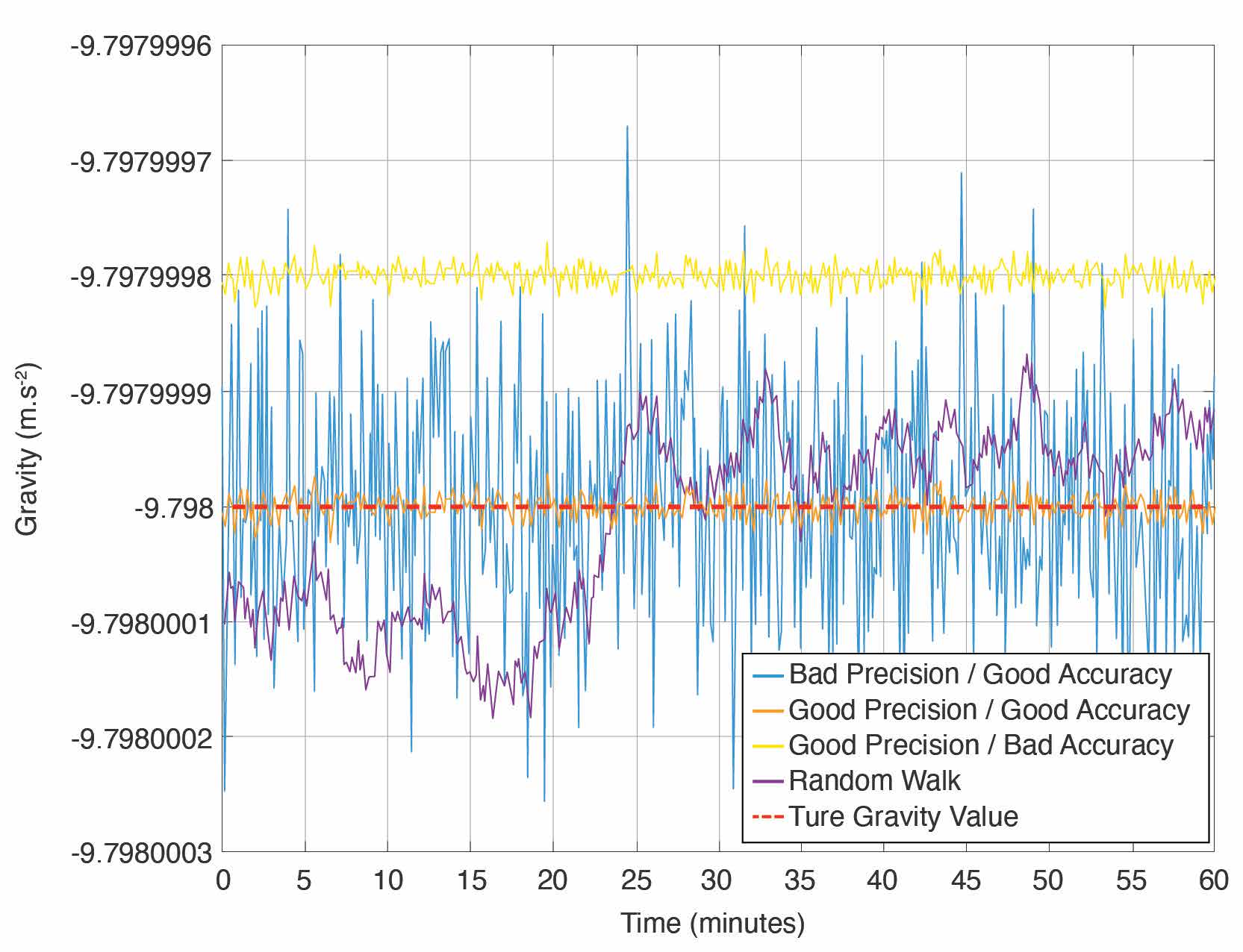
It is common to find gravimeters that have excellent precision and can make sensitive measurements of gravity over a short time but with bad accuracy. This typically manifests as a drift in the sensor over multiple hours and days. While this may sound detrimental, there are many scenarios where the long-term accuracy of a measurement is unimportant. For example, there is no need for long-term stability to map the presence of a small tunnel system. The measurements in Figure 2 were made with a device with excellent precision but no inherent accuracy. However, for the use case of monitoring the movement of mass underground, such as the levels of a concealed stockpile, it is essential to have a stable, accurate device so that any observed long-term changes can be attributed to a change in the stockpile level and are not just the drift of the sensor over time. This drift is demonstrated in Figure 7 (purple signal), where the gravimeter with random drift would be able to identify a mass change of 1,000 kilograms at a depth of 2 metres in a few minutes. However, it would be unable to track that change over hours due to the inherent drift of the sensor, which generates fictitious signals that mimic the subsurface mass change. To use the previous target shooting example, this is the zero of the sights drifting over time.

This leads to the question, ‘What is the minimum accuracy of a sensor?’ and, more precisely, ‘When is the minimum accuracy for a sensor achieved?’^[16] In this article, devices will be quantified by how well they can perform in a 100-second measurement. This gives a typical real-world survey precision and is a typical time needed to reach optimal precision of the CG‑6 gravimeter (the best precision commercial gravimeter). The best-in-class performance for different gravimeter technologies is shown in Table 2.

Figure 7: Various simulated gravimeter measurements over an hour. The purple data shows a random walk typical of relative gravimeters with good precision but a long-term accuracy drift. Such a sensor would, over a short time, be capable of identifying a mass void as small as 1,000 kilograms at 2 metres deep, but it would not be able to track changes over time.

Additional Challenges in Measuring Gravity

Simply because a gravimeter’s specifications might meet requirements, it does not mean that there are not other potential problems. There are three other critical limitations: firstly, the contamination of the gravity signal with motion of the platform or vehicle it is mounted on; secondly, the levelling requirements for a single-axis gravimeter; and finally, the altitude of the gravimeter as it moves through Earth’s gravity gradient.

The motion of the measurement platform matters; that is, if the gravimeter is mounted in a moving system such as an uncrewed aerial vehicle, movement of that vehicle will influence the gravity measurement. Physically, there is no way to differentiate between the acceleration signal of the sensor platform caused by its motion and that of the gravity signal from any surrounding density variations. This is why internal navigation calculations require a model of local gravity. This problem can often be overcome either through filtering of the signal, through use of a gravity gradiometer to reject the platform motion, or through an external position correction using a source such as GPS or lidar.

For a single-axis gravimeter, the device needs to be well aligned with local gravity, or the tilt will show as a reduction in gravity. For example, to measure a 10^‑7 m.s^‑2 signal, a single-axis gravimeter needs to be levelled to less than 0.01 degrees from vertical. This challenge can be overcome with level sensors but typically requires human involvement or complex active levelling systems.

The final challenge in measuring gravity is knowing the sensor altitude sufficiently well to remove the earth’s background gravitational gradient. The vertical gravitation gradient signal generated by the earth is approximately −3×10^‑6 s^‑2, meaning that for every metre of altitude a gravimeter gains, its measured gravity signal changes by −3×10^‑6 m.s^‑2 and therefore the measured signal needs to be compensated for this altitude shift. This puts a requirement on the necessary altitude measurement needed to resolve a specific gravitational signal. For example, if a device takes measurements over an area with a 0.1 m uncertainty in altitude, it will be unable to differentiate a gravitational signal below 3×10^‑7 m.s^‑2. To achieve measurements of gravity below 10^‑8 m.s^‑2, altitude must be known to a precision of 3 mm. The requirement to track altitude changes is the reason why an RTK GPS was used to take the data in Figure 2, and meeting the required altitude precision for the expected signal is needed in all gravimetric surveys. In commercial gravimetry surveys, this is commonly solved with GPS or a total station. 

Gravimeter Technologies

This section will break down the types of gravimeters by their underlying technology, using real-world examples in the commercial and research spaces. There is some historical uncertainty around the first measurements of gravity but the best known is the measurement made by Galileo Galilei, who measured gravity in the 16th century using a ball rolling down an inclined plane. Further measurements were performed by Eötvös using torsion pendulum-based devices in the early 20th century^[17] with demonstrations of detecting the gravitational pull of nearby mountains. Each technology will be described in the following subsections, and the best-in-class device specifications will be listed in Table 2.

Relative Gravimeter (Mass on a Spring)

Based on the solution to a university homework problem, Romberg and LaCoste developed spring-based gravimeters in 1931.^[18] These devices formed the basis for the modern relative gravimeter. The underlying principle of operation for these devices is that of a mass on a spring.^[19] Under the influence of earth gravity, the mass will pull on the spring and stretch it to a set displacement. If the acceleration of gravity changes, this displacement will change based on the known spring constant. Spring-based gravimeters are the most commonly used portable gravimeters and can typically be carried and operated by a single person, as seen in Figure 3. They can have incredible precision but lack accuracy and typically have bad long-term drifts. This makes them ideal for performing detection and mapping surveys, such as the work done with the CG‑6 gravimeter^[20] in Figure 2, but unsuitable for long-term subsurface monitoring applications.

Superconducting Gravimeter

Superconducting gravimeters, developed in the 1960s by Pothero and Goodkind, utilise the magnetic levitation of a spherical superconducting test mass.^[21] This design is an effective iteration of the classical spring-based gravimeter; however, the spring force is provided by a lossless superconducting electromagnet holding the superconducting sphere against gravity. The incredibly low loss of these systems means that they are the most sensitive of all gravimeter types ever built.

However, these devices have some severe disadvantages. Firstly, they must operate cooled by liquid helium (4 kelvin) and cannot be allowed to move above their critical temperature. Secondly, they are relative devices that can only measure changes in gravity. Lastly, they cannot be moved or altered in any way without fundamentally changing their operation set points. These limitations mean that superconducting gravimeters, while capable of reaching the necessary sensitivities for all applications, are unlikely to be of use in an Army context and there are no obvious technological pathways that would enable this technology type to become a portable sensor in the future.

Falling Corner Cube Gravimeter

The next technology to discuss is that of the ballistic free fall gravimeter. This was first developed by Faller in the 1950s^[22] and is based on the principle of dropping an object in a vacuum and measuring its position while undergoing free fall. To achieve world-class accuracy and precision, these devices require the position to be measured with an optical interferometer, where the falling object is a mirror that makes up part of the optical system. Niebauer developed the current generation of these devices,^[23] which have been the gold standard of gravimetry since the 1990s. The advantage of this technology is that it is inherently accurate, measuring the free fall of an object with reference to atomic clocks and atomically locked laser wavelengths. However, the devices are not easily portable, weigh over 100 kilograms and require technical expertise to set up and operate.

These devices meet both the precision and accuracy requirements for all discussed gravimetry applications. However, the existing commercial devices are bulky and difficult to use. They operate more like a small portable laboratory than a robust self-contained sensor. However, as discussed in literature,^[24] there are still possible improvements to be made in this technology space.

Cold Atom Interferometer Gravimeter

In the 1990s, when falling corner cube gravimeters were commercialised, the cold atom interferometer (CAI) gravimeter was pioneered by Kasevich and Chu.^[25] Using the experimental realisation of atoms that could be cooled down to near absolute zero, Kasevich and Chu demonstrated that these small clouds of cold atoms could be used as the test mass for a gravimetric sensor. It should be noted that cold atoms provide no inherent advantage in measuring gravity, as the universality of free fall means that any dropped mass will accelerate equally.

This type of gravimeter has been one of the primary focuses of quantum sensor research. However, there are many parallels between the cold atom gravimeters and the falling corner cube gravimeters. Both commercial offerings of these devices are large portable laboratory type devices, reaching similar levels of precision and accuracy. The quantum nature of these devices has not yet shown a significant improvement over the previous technology for a commercial device.

One area where cold atoms have a clear technological advantage is in the construction of a gravity gradiometer, where a single interferometer laser can operate on multiple atomic clouds to remove systematic effects.^[26]

Much of today’s gravimetry focus is on this technology, and it is considered a favourable competitor for pushing the field forward. However, it should be noted that the complexity overhead of laser cooling atoms should not be underestimated. Until a commercial entity can show a maintenance-free portable sensor, they are unlikely to see use in the land forces.

Micromechanical Gravimeters

Lastly, it would be remiss not to discuss the fields of micromechanical devices. Encompassing optical resonator readouts, mass on springs, optically levitated nanoparticles and micro-electromechanical systems (MEMS), this is the most widely varying field of gravimeter/accelerometer. Your smartphones contain a three-axis MEMS accelerometer capable of measuring gravity; however, it is neither accurate nor precise enough to measure subsurface signals like the ones discussed in this article.

Recent work in this field suggests that these micromechanical devices may be able to compete with the mass-on-a-spring gravimeters discussed earlier. This is a potentially fruitful field that could leverage the existing silicone processing chain to manufacture smaller and cheaper devices.^[27] 

Table 2. Specifications for each gravimeter technology that is the current best in class, to the nearest order of magnitude (published data). 

Technology	Type	Precision at 100 s (m.s‑-2)	Long-term survey	Weight / portable
Spring[28]	Relative	10‑8	No	8 kg / yes
Falling corner cube[29]	Absolute	10‑8	Yes	100 kg / with setup
Superconducting[30]	Relative	10‑10	Yes*	100 kg / no
Atom interferometer[31]	Absolute	10‑8	Yes	100 kg / with setup
Micromechanical[32]	Relative	10‑7	No	5 kg / yes

* Superconducting gravimeters are only capable of long-term surveys in a single measurement run.

Table 2 shows the current state of the art for these gravimeter technology types, and should be considered in conjunction with Figure 8. It can be seen that for most technology types, a limit of about 10^‑8 m.s^‑-2 in a 100-second integration has not yet been beaten. Part of this probably relates to the fundamental microseism noise and the sea of problems around 10^‑10 m.s^‑-2. However, there is no fundamental science limiting these devices, and in existing applications, measuring at this level of precision and timeframe is adequate.

The other factor here is the size, weight and power (SWaP) of gravimeters. Looking at Figure 8, one might think that emerging technologies like CAI and MEMS gravimeters hold no benefit, but of course precision, while critical, is only part of the story. Some of the biggest gains to be made in gravimeter technology are in reducing the weight, size and complexity of these devices. Today, all commercial absolute gravimeters are effectively small portable laboratories that require a skilled operator. This will change with improved technology, and one of the key development areas for Army will be in the reduced form factor and ease of use that future devices will bring.

Figure 8: Development timelines of gravimeters in precision (top) and weight (bottom). All gravimeter technologies except for superconducting types begin to hit a limit of around 10^‑8 m.s^‑2. While further work could be done to push this precision, the applied use cases for these small signals are questionable and any sensor capable of short-term precision below 10^‑6 m.s^‑2 is of potential use. The more telling development factor is the improvement in weight and inherent portability. The red-shaded area indicates the ideal ground for sensor development, where the reduced form factor would be a key enabler for potential Army use cases. Some weights are estimated based on materials and photographs. 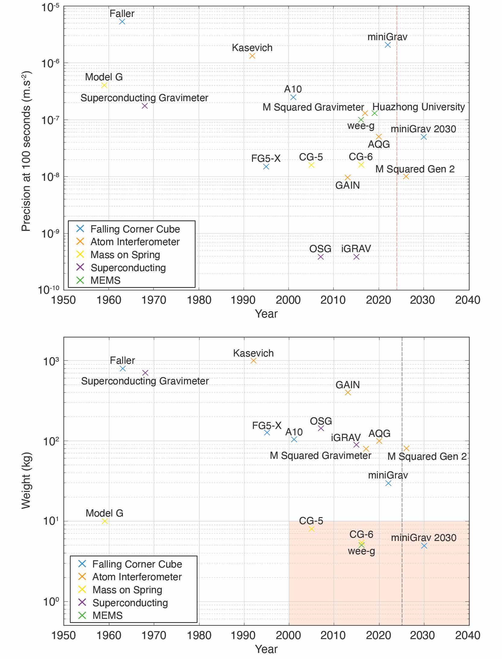References: Faller,^[33] FG5‑X,^[34] A10,^[35] MiniGrav,^[36] Kasevich,^[37] GAIN,^[38] M Squared,^[39] AQG,^[40] Model G,^[41] CG‑5,^[42] CG‑6,^[43] Superconducting Gravimeter,^[44] OSG,^[45] iGrav,^[46] wee‑g,^[47] Huazhong University.^[48] 

Conclusion

This article has demonstrated applications for which gravimetry could be used in Army and has identified subsurface detection and monitoring as the best candidate for success. Impact and real-world measurements were taken to demonstrate this application utilising existing commercial sensors. Gravity detection is a unique sensing modality that cannot be blocked or jammed and is very difficult to fake. Its addition could be a valuable tool to augment existing subsurface detection methods, enhancing the utility of magnetometers, ground-penetrating radar and exploratory digging.

The underlying physical principles behind gravity measurements were explored, showing the expected signal strengths for various subsurface anomalies, and sensible limits were put on what could be physically achieved. Finally, various technology streams for different gravimeter types and their ongoing development have been investigated, showing a common trend where precision plateaus at the useful limit, but newer technology is making significant advances in reducing the SWaP of these sensors.

The most effective way to progress this technology within Army is to begin testing and using the current-day technology in field trials of the various applications. Commercial industry has already done the development work to build commercially available gravimeters capable of these applications. What is lacking is knowledge and experience in defence to apply and test these applications. Once clear use cases and applications are established, Army can feed back into the research and development pipeline with more explicit problem statements and specifications to refine particular use cases.

About the Author

Dr Samuel Legge is an experimental research physicist and Australian Army Research Centre Fellow (2023) working in the Research School of Physics at the Australian National University. He is part of the quantum sensors research group and specialises in lasers, quantum sensor development, experimental design, and fabrication.

Endnotes

^[1] M Schwirtz, ‘Last Stand at Azovstal: Inside the Siege That Shaped the Ukraine War’, The New York Times, 24 July 2022.

^[2] ITA-AITES, Tunnel Market Survey 2019, at: https://nff.no/wp-content/uploads/sites/2/2021/01/Market-Survey-2019.pdf.

^[3] Muquans, ‘Absolute Quantum Gravimeter’, Muquans (website), at: Talence, France, [Online]. Available: https://www.muquans.com/product/absolute-quantum-gravimeter/ (accessed 6 November 2024).

^[4] Scintrex, CG‑6 Autograv Gravity Meter Operation Manual: Rev B (Concord, 2018).

^[5] Emlid, REACH M2/M+/RS2/RS2+ User Documentation (Budapest, 2023).

^[6] See the ‘Measuring Gravity’ section of this article to understand the relevance of these numbers and the ‘Gravimeter Technologies’ section for details regarding the CG‑6 gravimeter.

^[7] Scintrex, CG‑6 Autograv Gravity Meter Operation Manual.

^[8] FW Landerer et al., ‘Extending the Global Mass Change Data Record: GRACE Follow‐On Instrument and Science Data Performance’, Geophysical Research Letters 47, no. 12 (2020), at: https://doi.org/10.1029/2020GL088306.

^[9] Australian Government, National Defence: Defence Strategic Review 2023 (Canberra: Commonwealth of Australia, 2023), at: https://www.defence.gov.au/about/reviews-inquiries/defence-strategic-review.

^[10] X Wang  et al., ‘Improving Measurement Performance via Fusion of Classical and Quantum Accelerometers’, The Journal of Navigation 76, no. 1 (2023): 91–102.

^[11] ‘Microgravity’, RSK Geosciences (website), at: https://rskgeosciences.co.uk/services/geophysical-surveys/techniques/microgravity.

^[12] M Anderson et al., Where Is All the Water?, report to the NSW Government report, (Sydney: NSW Smart Sensing Network (, 2021).

^[13] ‘A Year-Long Field Campaign on Mount Etna to Prove the Absolute Quantum Gravimeter Value for Volcanology’, Exail (website), 7 July 2022, at: https://www.exail.com/resources/customer-stories/a-year-long-field-campaign-on-mount-etna-to-prove-the-absolute-quantum-gravimeter-value-for-volcanology (accessed 7 February 2024).

^[14] Of the nine total gravity gradient values, only five are independent.

^[15] JE Faller, ‘The Measurement of Little g: A Fertile Ground for Precision Measurement Science’, Journal of Research of the National Institute of Standards and Technology 110, no. 6 (2005): 559–581.

^[16] For those who want the full picture of this complicated topic, the term to research is known as Allan deviation.

^[17] L Bod, E Fischbach, G Marx and M Náray-Ziegler, ‘One Hundred Years of the Eötvös Experiment’, Acta Physica Hungarica 69 (1991): 335–355.

^[18] RD Clark, ‘University of Texas, Lucien Jean Baptiste LaCoste, August 25, 1907–March 8, 1995’, UT Physics Department History (website), at: https://www.utphysicshistory.net/LucienLaCoste.html (accessed 20 October 2024).

^[19] L LaCoste, ‘A New Type Long Period Vertical Seismograph’, Journal of Applied Physics 5 (1934): 178–180.

^[20] Scintrex, CG‑6 Autograv Gravity Meter Operation Manual.

^[21] JM Goodkind, ‘The Superconducting Gravimeter’, Review of Scientific Instruments 70 (1999): 4131–4152.

^[22] Faller, ‘The Measurement of Little g’.

^[23] ‘About Us’, Micro-g LaCoste (website), at: https://microglacoste.com/about (accessed 20 October 2024).

^[24] Faller, ‘The Measurement of Little g’.

^[25] Mark Kasevich and Steven Chu, ‘Atomic Interferometry Using Stimulated Raman Transitions’, Physical Review Letters 67, no. 181 (1991).

^[26] B Stray  et al., ‘Quantum Sensing for Gravity Cartography’, Nature 602 (2022): 590–594.

^[27] RP Middlemiss et al.,GD Hammond, ‘Measurement of the Earth Tides with a MEMS Gravimeter’, Nature 531 (2016): 614–617.

^[28] Scintrex, CG‑6 Autograv Gravity Meter Operation Manual.

^[29] Micro-g LaCoste, FG5-X Absolute Gravimeter User’s Manual: Release 115-060-001A.01 (Lafayette, USA2015).

^[30] ‘iGrav Gravity Sensors’, GWR Instruments, Inc (website), at:  San Diego, United States of America, [Online]. Available: https://www.gwrinstruments.com/igrav-gravity-sensors.html (accessed 6 November 2024).

^[31] C Freier, ‘Atom Interferometry at Geodetic Observatories’, PhD thesis, Humboldt-Universität zu Berlin, 2017, at: https://doi.org/10.18452/17795.

^[32] Middlemiss et al., ‘Measurement of the Earth Tides with a MEMS Gravimeter’.

^[33] JE Faller, ‘An Absolute Interferometric Determination of the Acceleration of Gravity’, PhD thesis, Princeton University, 1963.

^[34] Micro-g LaCoste, FG5-X Absolute Gravimeter User’'s Manual.

^[35] Micro-g LaCoste, A-10 Portable Gravimeter User’s Manual (Lafayette, USA2008).

^[36] ‘MiniGrav: Drone Deployable Miniturised Absolute Gravimeter’, Australian National University (website), at: https://research.anu.edu.au/partner-with-us/technology-marketplace/minigrav-drone-deployable-miniturised-absolute-gravimeter (accessed 27 August 2024).

^[37] Kasevich and Chu, ‘Atomic Interferometry Using Stimulated Raman Transitions’.

^[38] Freier, ‘Atom Interferometry at Geodetic Observatories’.

^[39] M Squared, at: 
 https://web.archive.org/web/20260310055910/ https://m2lasers.com/quantum-gravimeter.html.

^[40] Muquans, ‘Absolute Quantum Gravimeter’.

^[41] LaCoste & Romberg, Inc, Instruction Manual Model G&D Gravity Meters (Austin, USA2004).

^[42] Scintrex, CG‑6 Autograv Gravity Meter Operation Manual.

^[43] Ibid.

^[44] WA Prothero and JM Goodkind, ‘A Superconducting Gravimeter’, Review of Scientific Instruments 39, no. 9 (1968): 1257–1262.

^[45] GWR Instruments, Inc, Operating Principles of the Superconducting Gravity Meter, at: https://www.gwrinstruments.com/pdf/principles-of-operation.pdf (accessed 6 November 2024).

^[46] GWR Instruments, Inc, ‘iGrav Gravity Sensors’.

^[47] Institute for Gravitational Research, School of Physics and Astronomy, University of Glasgow, Wee-g.com, at: https://wee-g.com (accessed 6 November 2024).

^[48] S Tang et al. and , ‘A High-Sensitivity MEMS Gravimeter with a Large Dynamic Range’, Microsystems & Nanoengineering 5, no. 45 (2019), at: https://doi.org/10.1038/s41378-019-0089-7.